Presentation:

The purpose of this page is to show the reflection of horn with an experimental device.

Explanation of the device:

The principle of this device is to delay the reflection, making it take a longer path in order to isolate it in time.

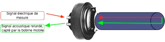
For this he was inserted a tube of 1 meter between the transducer and the horn, as shown in illustration No. 1:

The measure will be made with LogSweep signal to the terminals of the transducer itself and will supersede to a microphone measurement.

This will measure only what happens in the tube, ie the reflection has the mouth of the device.

The acoustic energy reflected out of the assembly returns to the voice coil with a delay, as outlined in the illustration No. 2.

Illustration n°2

For 1 meter of pipe we have an echo that comes with 6ms of delay after the signal measurement.

These 6ms correspond to the time it takes for sound to travel 2 meters, ie to make a return trip in the tube of 1 meter.

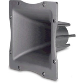
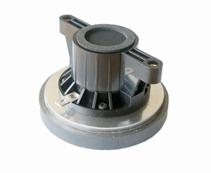
The transducer used is the BMS 4524 and the horn is a RCF HF101.

Measures:

In the illustration No. 3 we see that after 6ms, the first echo on a bare tube recessed.

This measure in single tube will serve as a comparison with the tube bearing the horn at its mouth.

In the illustration No. 4 we see a minimum of 8 echoes, spaced 6ms, whose amplitude is inceasingly low,  which are captured by the transducer:

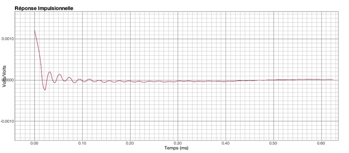
Illustration No. 5 shows the impulse responses of single tube and tube with horn. They reflect the unique impedance of the transducer and therefore are identical and overlap perfectly

In the illustration No. 6 we see the impedance curves in dB corresponding to the impulses of the illustration No. 5 with a window for a period of 6ms from the beginning of the pulse.

Not surprisingly, they are identical and are overlap as well:

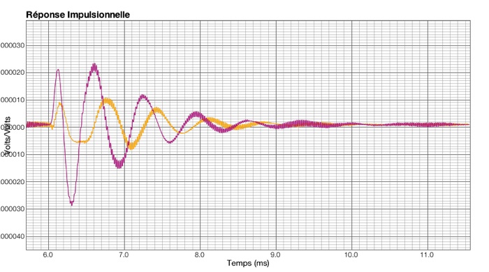
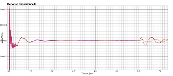
6ms after, we see in the illustration No. 7 the first echoes with the HF 101 and single tube, they do not return the same signal to the transducer.

Illustration No. 8 shows a zoom of the firsts echoes:

These energy captured are not identical and overlap, they will therefore have different amplitudes curves.

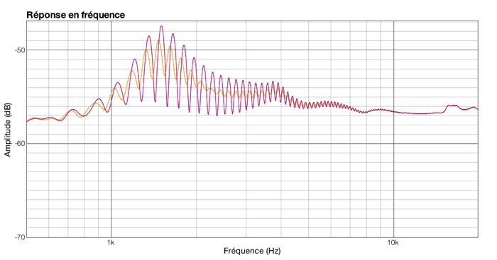
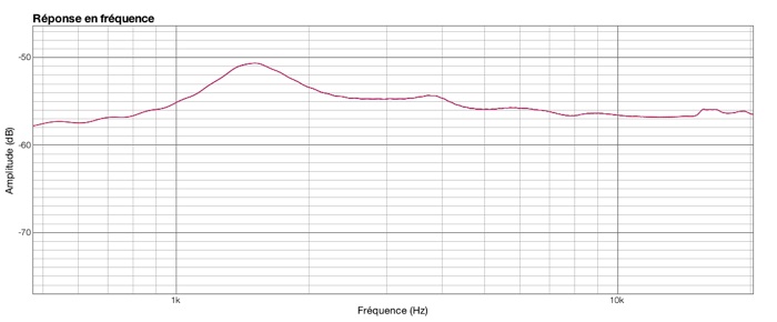
In the illustration No. 9, curves of amplitude with a window for a period of 6ms from the beginning of the echo:

We observe that the presence of the horn has the mouth of the tube (orange curve) reduced to twenty decibels the amount of energy that returns to the acoustic transducer.

However, on the approach of the cutoff frequency of the horn given to 1000Hz, the reflected energy is increasing rapidly.

The drop in level before 1500Hz, due to the natural cutoff of the transducer below its resonant frequency, so there is less energy captured in return.

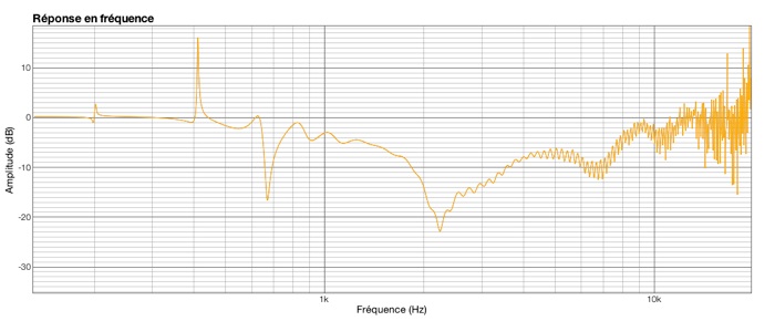
In the illustration No. 10, we have a curve that shows the difference in amplitude between the first echo with and without the horn on the device.

Below 2KHz, we see that the difference tends to disappear gradually in spite of some very localized accident frequency, which means that the amount of diffracted energy tends to be identical in both cases.

We note above 8KHz a difference that also tends to zero, but this time for the opposite reason, there is very little energy diffracted at these frequencies in both cases and therefore a little energy back (on the shown in the illustration No. 9).

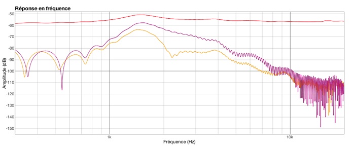
If included in the time window the main pulse and first echo, we obtain different impedance curves of the illustration No. 6, as shown in illustration No. 11:

We see that more reflection is low (with a horn), more the impedance curve is smooth.

Conclusion:

We observe that only the reflection alters and disrupts the impedance curve because when the experiment described in this document, the first 6 milli-seconds of the impulse response are unchanged despite the presence or absence of a horn at the end of tube.

The presence of reflection shows that the horn no longer plays its role as adapter acoustic impedance becomes reactive.

It can not therefore be considered a horn since it does not fulfill its primary function, that of transmitting sound.

However, in practice the horn are not infinite, which implies a natural cut-off frequency.

They very quickly become reactive (Figure No. 9) has the approach of their frequency.

This leads to a propagation delay time acoustic group not constant at these frequencies is the effect of the sum of the echoes (limited bandwidth), which leads to a global delay of the signal.

This explains why the measured emissive center, has the approach of cut-off frequency of horn, is much more backward than the physical position of the transducer.

What is true with the cutoff frequency is also with the diffraction horn, ie not just reactive to the acoustic cut-off.

The effects are similar to the response curve for the acoustic impedance curve (Figure No. 11): we have a comb filter response.

This shows that the main function of a horn is to not diffract offering an acoustic impedance resistive over a bandwidth as wide as possible.

The second function is to obtain a compatible directivity with listening of sound and music, but this is not the subject of this page.

Illustration n°7

Illustration n°8

Illustration n°9

Illustration n°10

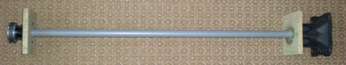
Illustration n°11

Illustration n°1

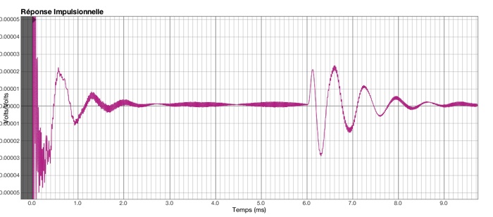
Illustration n°3

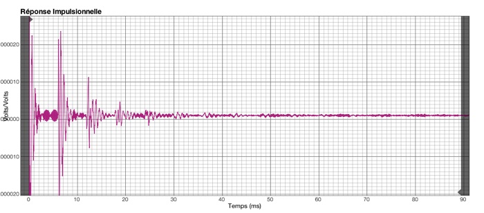
Illustration n°4

Illustration n°5

Illustration n°6

Measure signal

acoustic signal delayed and captured by the coil.

See also Kundt’s tube.